Crisp and Interval-Based Conditional Probabilities
“Censored data” is the common statistical term for values that are within an interval. A typical example from environmental data-sets are measurements below a certain detection limit. If a measurement is below detection limit, due to the analytical performance of the device that measures the concentration, we don’t know its precise value, but we do know that it is somewhere in the interval \[\smash{\in(0, \textnormal{detection limit})}\].
Application in Environmental Hydrology
A typical example where censored measurements play an important role are solute concentrations in groundwater. The measured concentration value of some solute depends on the analytical method that was used for quantification of the concentration. Sometimes, the concentration is so small that we can not be certain about it’s value, and we assume that the true value is somewhere between zero and the analytical detection limit.
In a recent example, my coauthors and I demonstrated the importance of including censored measurements to derive a representative concentration of chlorinated solutes in a hydrogeological layer at two boreholes within a fractured sandstone. Due to the fractured nature of the sandstone, at most depths the concentrations were fairly small and frequently below detection limit, whereas in the fractures, typically large concentrations were encountered. Taking the censored measurements (the concentrations below detection limit) in a statistical meaningful way into account lead to an estimate of representative concentrations that corresponded to the conceptual site hydrogeological model at the upstream and downstream borehole, and can be important for site assessment.
Related to censored measurements, but different, are true zeros. An example of a measurement of true zero is a rain gauge that measures precipitation when it does not rain. The distinction between a true zero and a measurement below detection limit can be tricky, because they are both small values. If you’re interested in how to include true zeros in this approach, please continue to read here. A truely zero measurement means that its value is zero and not in an interval between zero and the detection limit.
If you are interested in a statistically reasonable treatment of censored measurements, you can find the related publication in Environmental Science and Technology.
I’ll explain the basic underlying theory below.
Basic Statistics Example
I have written about conditional_probabilities quite some time ago. This can be viewed as an extension.
A crisp condition is something like “what is the probability of event A to occur, given event B has occurred”. This is how conditional probabilities are typically taught with. Compared to a univariate density, a conditional density should have a smaller variance, and is shifted towards the condition. So far so good.
It turns out that there is a “not-crisp” condition. This is something like “probability of event A given that ‘event’ B is somewhere between zero and b”. The funny thing is, that the uncertainty about this event to occur is smaller than a corresponding normally-distributed univariate event.
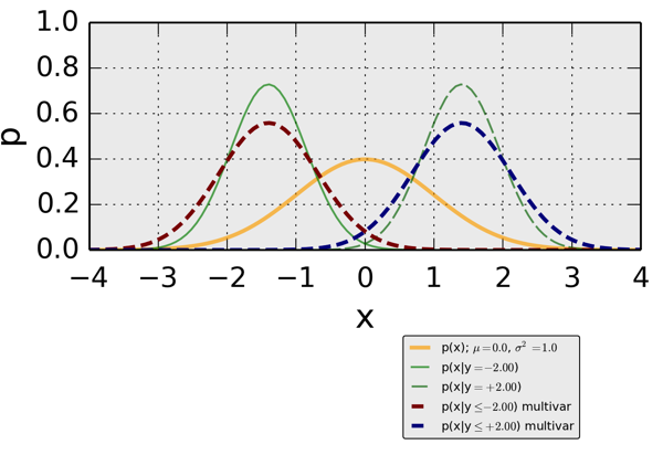
When looking at the figure below, this means:
- the yellow line indicates a standard (variance=1) normal Gaussian density
- two crisp conditional densities are shown by the solid (\[p(x|y=-2.0)\]) and the dashed (\[p(x|y=+2.0)\]). Both those densities have a smaller uncertainty (variance) than the univariate standard normal
- two interval-based conditional densities are shown in red (\[p(x|y \leq -2.0)\]) and blue (\[p(x|y \leq +2.0)\]). The interval-based densities have the same location as the crisp conditionals. Their uncertainties are smaller than the corresponding univariate, but larger than the crisp conditionals.
